Unsupervised learning for mapping of spatial gene expression data
Introduction / Abstract
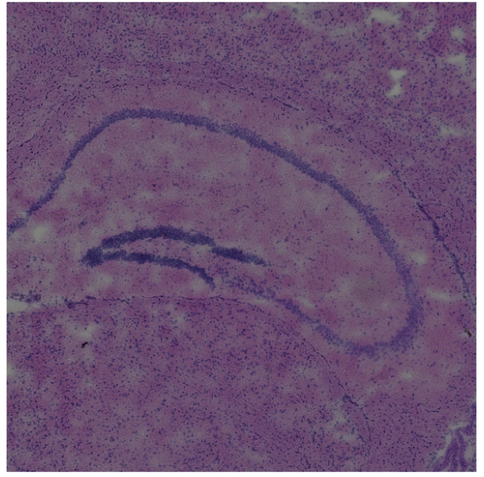
In this exploratory project, I used a machine learning pipeline to analyse 10x Visium sample data of mouse brain section
I used Principal Component Analysis (PCA) for dimensionality reduction of the gene expression features and graph-based clustering algorithms to reconstruct the tissue structure, without using spatial labelling data. I used differential expression analysis to validate the proposed structure, which coherently returned C1ql2 as the marker for the proposed region corresponding to the Dentate Gyrus.
Tech Stack

Python 3.9

Scanpy

Squidpy

Matplotlib
Data Preprocessing
Spots with less than 500 distinct genes were filtered out as noise.
Spots with at least 20% mitochondrial reads were also filtered out as they are indicative of cell death.
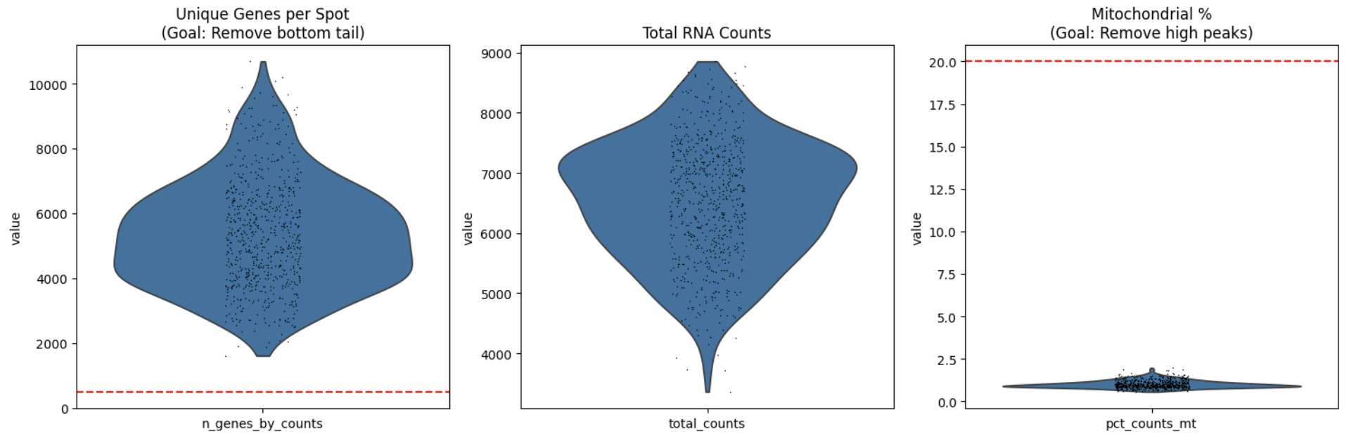
Counts were normalised to 10,000 and a natural log + 1 transformation was applied to address heteroscedasticity and effectively coerce multiplicative fold-changes into additive changes, necessary for subsequent Euclidean distance calculations.
Dimensionality Reduction
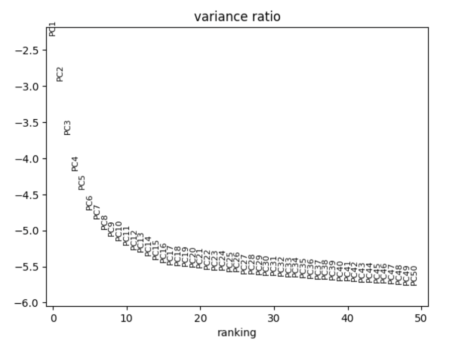
The dataset runs into the issue of the curse of dimensionality since each spot has about 20,000 distinct genes. Therefore, feature selection was performed by selecting the top 2,000 Highly Variable Genes. Then, Principal Component Analysis was used to compress these feature into 40 "eigen-genes".
Graph-based clustering
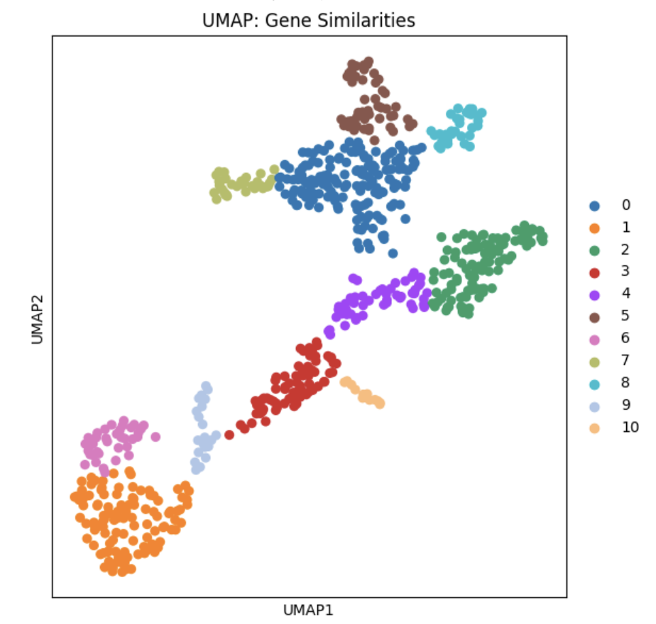
With a now tractable dimension, a kNN graph (k = 10) was constructed using the PCA space. Then, the Leiden Algorithm (resolution 0.8) was used for community detection.
Results and validation
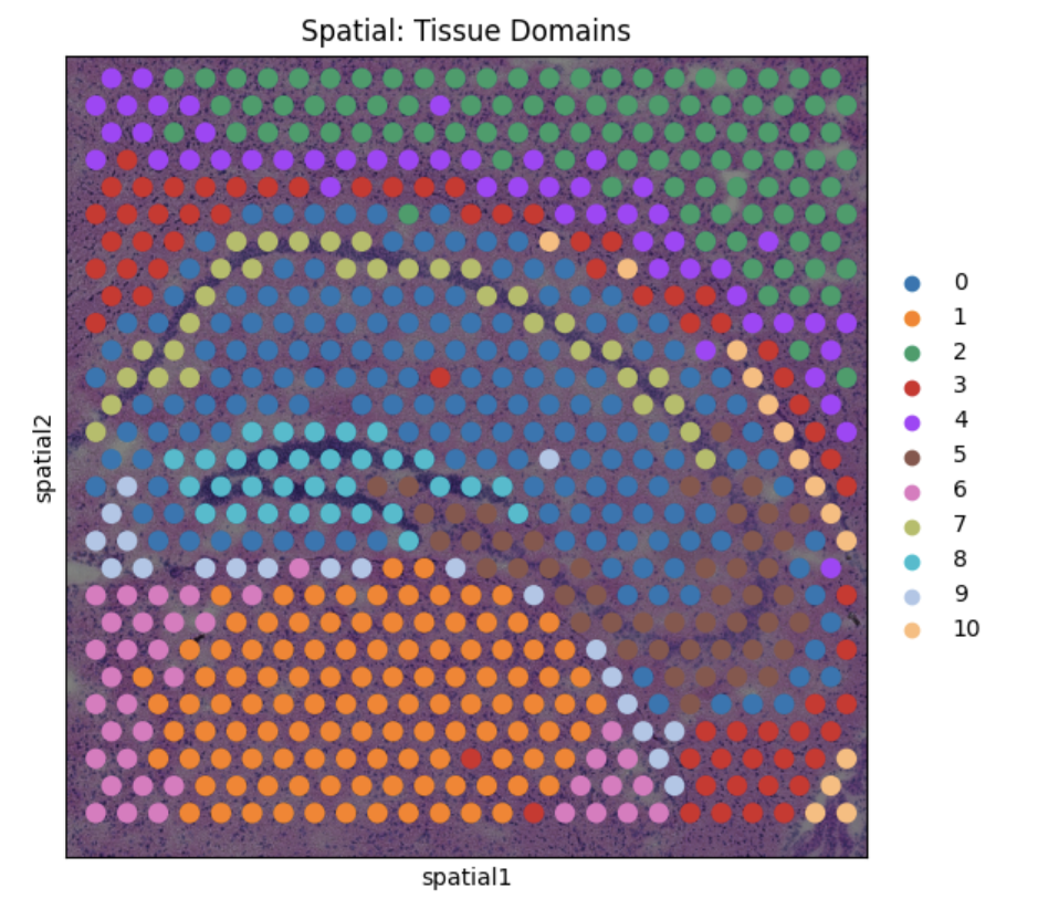
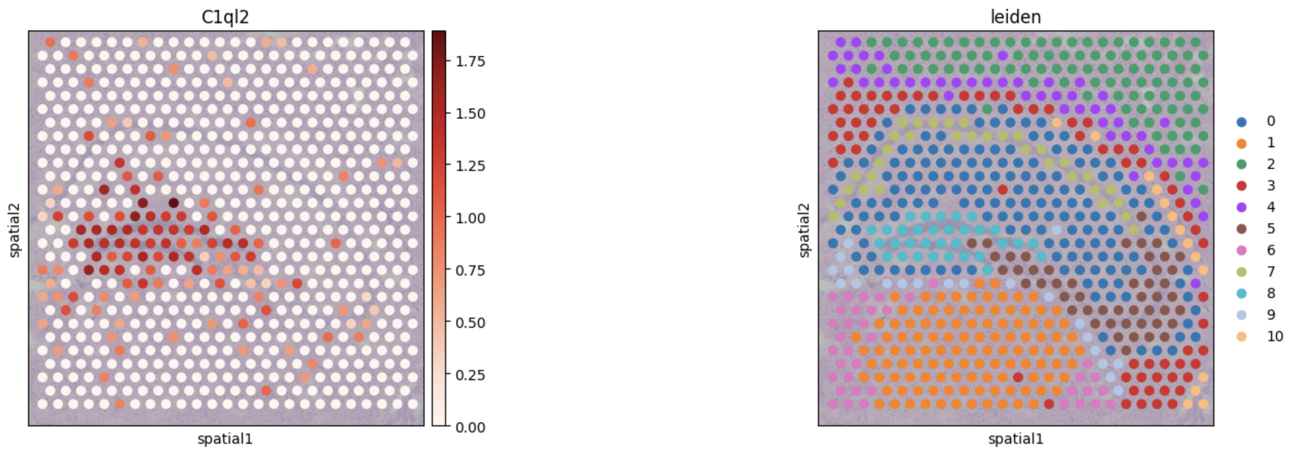
In spite of the fact that these steps did not incorporate the use of spatial coordinate information, the algorithms successfully partitioned the tissue into sections visually coherent with the histological image. In particular, Cluster 8 forms the distinct C-shaped structure of the Dentate Gyrus.
To further validate the identification of this region, differential expression analysis using a "One vs Rest t-test" was conducted. The C1ql2 gene was identified as the most significantly different marker when compared to other clusters. Since C1ql2 is a known marker of the Dentate Gyrus, we can therefore confirm both visually and biologically that the algorithm pipeline had correctly identified the Dentate Gyrus.
Conclusion
This exploratory project demonstrated that unsupervised machine learning methods have the potential to reconstruct and identify structures in histological images by processing sequencing reads. This is an important application in spatial transcriptomics as automated annotation enables the future of automated digital pathology.